seqlogit: Stata module to fit a sequential logit model
Author: Maarten L. Buis
seqlogit fits a sequential logit model. This model is know under a variety of other names: sequential logit model (Tutz 1991),sequential response model (maddala 1983), continuation ratio logit (Agresti 2002), model for nested dichotomies (fox 1997), and the Mare model (shavit and blossfeld93) (after (Mare 1981)).
A sequential logit model can be estimated quite simply by estimating a number of logit models. The seqlogit package serves three additional purposes: First, it makes it easier to test hypotheses across transitions since the entire model is estimated simultaneously. Second, it implements the decomposition proposed by Buis (2010) of the effect of an explanatory variable on the outcome of the process described by the sequential logit into the contributions of each of the transitions. Third, it implements and extends the strategy proposed by Buis (2011) of doing a sensitivity analysis to investigate the potential influence of unobserved variables.
For this last purpose, the seqlogit package allows one to estimate a sequential logit given a scenario concerning the unobserved variables. These effects will only be estimated when the sd() option is specified. A regular sequential logit model, which assumes that there is no unobserved heterogeneity, is estimated if the sd() option is not specified. The scenarios assume that these unobserved variables either add up to a standardized normally (Gaussian) distributed variable (when the pr() is not specified), or to a standardized discrete variable (when the pr() is specified). The effects of this aggregate unobserved variable during each transition are specified in the sd() option. The correlation during the first transition between this unobserved variable and the variable specified in the ofinterest() option is specified in the rho() option. The scenarios are estimated using maximum simulated likelihood, while the regular sequential logit model is estimated using regular maximum likelihood.
Supporting materials
- article introducing the decomposition implemented in seqlogit.
- article introducing the scenarios implemented in seqlogit.
- summary on ssc.
- helpfiles:
- Announcement of seqlogit on statalist.
- Certification script I used for checking the latest version of seqlogit (version 1.1.13).
References
Agresti, Alan 2002, Categorical Data Analysis, 2nd edition. Hoboken, NJ: Wiley-Interscience.
Buis, Maarten L. 2010, Not all transitions are equal: The relationship between inequality of educational opportunities and inequality of educational outcomes. in: Maarten L. Buis, Inequality of Educational Outcome and Inequality of Educational Opportunity in the Netherlands during the 20th Century. link
Buis, maarten L. 2011, "The Consequences of Unobserved Heterogeneity in a Sequential Logit Model", Research in Social Stratification and Mobility, 29(3), pp. 247-262. link
Fox, John 1997, Applied Regression Analysis, Linear Models, and Related Methods. Thousand Oaks: Sage.
Maddala, G.S. 1983, Limited Dependent and Qualitative Variables in Econometrics. Cambridge: Cambridge University Press.
Mare, Robert D. 1981, Change and Stability in educational Stratification, American Sociological Review, 46(1): 72-87.
Shavit, Yossi and Hans-Peter Blossfeld 1993, Persistent Inequality: Changing Educational Attainment in Thirteen Countries Boulder: Westview Press.
Tutz, Gerhard 1991, Sequential models in categorical regression, Computational Statistics & Data Analysis, 11(3): 275-295.
examples
Table of content
- When one can assign values to each outcome
- When it is not possible to assign values to each outcome
- Using marginal effects instead of log odds ratios
When one can assign values to each outcome
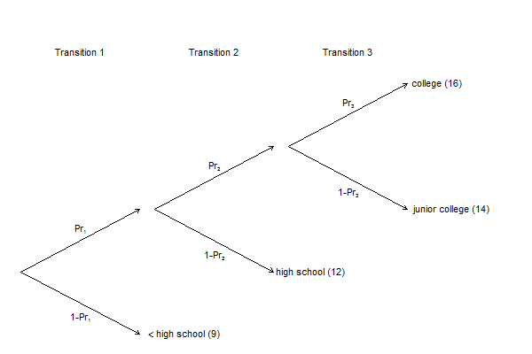
Consider the following simplified version of the American educational system. It consists of three transitions: First you decide whether you finish high school or not, than given that you finished high school you decide whether you get some college or not, and finally given that you decided to take some college you decide whether you go to a junior college or a full college. With seqlogit you would model how various explanatory variables influence these three transition probabilities.
That model can also be used to study how these explanatory variable influence the highest achieved level of education. Moreover, it can be used to relate the effects on the individual transitions to the effect on the final outcome.
The first step is to see that transition probabilities together with the values attached to each outcome define the expected value of the final outcome. From the transition probabilities we can derive the probabilities for each outcome: e.g. The probability of getting less than high school is 1-Pr1, and the probability of attaining only high school is Pr1×(1-Pr2), etc. I have assigned a value to each level of education (less than high school = 9, high school = 12, junior college = 14, college = 16). So, the expected highest achieved level of education is:
E(outcome) = (1-Pr1)×9 + Pr1×(1-Pr2)×12 + Pr1×Pr2×(1-Pr3)×14 + Pr1×Pr2×Pr3×16 (1)
The sequential logit model models how the transition probabilities differ between individuals1 with different values on the explanatory variables, so it also models how the expected outcome differs between these individuals. we can see how much E(outcome) changes when one of the explanatory variables changes by computing the first derivative of equation (1) with respect to these explanatory variables. These explanatory variables are present in equation (1) in the sense that the Prks in equation (1) are thus functions of the explanatory variables. It turns out2 that this derivative implies a meaningful relationship between the effects on the different transitions and the effect on the final outcome:
∂E(outcome)/∂x = ∑ ( at riskk × variancek × gaink ) βk (2)
In this equation x is the explanatory variable, at riskk the proportion of persons at risk of passing transition k, variancek is the variance of the dependent variable for transition k, that is, Prk(1-Prk), gaink is how much a person can expect to gain from passing transition k, and βk is the effect of variable x on the log odds of passing transition k. So the total effect is a weighted sum of the effects on each transition, and a transition receives more weight when more people are at risk,it is not the case that virtually everybody passes or virtually everybody fails that transition, and people can expect to gain much from passing that transition.
It is the use of this relationship between the effect on the transitions and the effect on the final outcome that is the main purpose focus of seqlogit and in particular seqlogitdecomp. To illustrate this one first needs to estimate a sequential logit model, as is done below.
. set lstretch off
. use "http://fmwww.bc.edu/repec/bocode/g/gss.dta", clear (General Social Surveys, 1972-2004 [Cumulative File])
. . recode degree 4=3 (degree: 870 changes made)
. label define degree 0 "lt high school" /// > 1 "high school" /// > 2 "junior college" /// > 3 "college", modify
. label value degree degree
. . gen byte res16 = 1*country + 2*town + 3*suburb + 4*city (18 missing values generated)
. label define res16 1 "country" /// > 2 "town" /// > 3 "suburb" /// > 4 "city"
. label value res16 res16
. . replace coh = coh - 5 (13421 real changes made)
. label var coh "(year of birth-1950)/10"
. . seqlogit degree south i.res16 c.sibs##c.sibs /// > c.coh##c.coh if black == 0 , or /// > tree(0 : 1 2 3 , 1 : 2 3 , 2 : 3 ) /// > ofinterest(paeduc) /// > over(c.coh##c.coh) /// > levels(0=9, 1=12, 2=14, 3=16)
Transition tree:
Transition 1: 0 : 1 2 3 Transition 2: 1 : 2 3 Transition 3: 2 : 3
Computing starting values for:
Transition 1 Transition 2 Transition 3
Iteration 0: log likelihood = -8004.1209 Iteration 1: log likelihood = -8004.1209
Number of obs = 8605 LR chi2(33) = 2545.09 Log likelihood = -8004.1209 Prob > chi2 = 0.0000
------------------------------------------------------------------------------ degree | Odds Ratio Std. Err. z P>|z| [95% Conf. Interval] -------------+---------------------------------------------------------------- _1_2_3v0 | south | .4967571 .0427537 -8.13 0.000 .4196478 .588035 | res16 | 2 | 1.10804 .1042108 1.09 0.275 .9215106 1.332327 3 | 1.351188 .232949 1.75 0.081 .9637534 1.894373 4 | .9760781 .142089 -0.17 0.868 .7337938 1.29836 | sibs | .7422851 .0433183 -5.11 0.000 .6620584 .8322335 | c.sibs#| c.sibs | 1.010062 .0053602 1.89 0.059 .9996109 1.020623 | coh | 1.182719 .1257414 1.58 0.114 .9602529 1.456725 | c.coh#c.coh | .9621042 .0442163 -0.84 0.401 .8792304 1.052789 | paeduc | 1.230506 .0184658 13.82 0.000 1.194841 1.267236 | c.paeduc#| c.coh | 1.001602 .0102535 0.16 0.876 .9817059 1.021902 | c.paeduc#| c.coh#c.coh| .9944196 .0047478 -1.17 0.241 .9851575 1.003769 | _cons | 5.772305 1.221072 8.29 0.000 3.813171 8.738004 -------------+---------------------------------------------------------------- _2_3v1 | south | .9735429 .0568136 -0.46 0.646 .8683224 1.091514 | res16 | 2 | .9071416 .0591979 -1.49 0.135 .7982293 1.030914 3 | 1.188069 .1003155 2.04 0.041 1.006862 1.401888 4 | .8392813 .0791339 -1.86 0.063 .6976694 1.009637 | sibs | .7501739 .0269693 -8.00 0.000 .6991344 .8049396 | c.sibs#| c.sibs | 1.018469 .0040838 4.56 0.000 1.010496 1.026505 | coh | .9466328 .0824247 -0.63 0.529 .7981162 1.122786 | c.coh#c.coh | .9759243 .0479077 -0.50 0.620 .8864027 1.074487 | paeduc | 1.226367 .0122549 20.42 0.000 1.202582 1.250623 | c.paeduc#| c.coh | 1.014192 .006924 2.06 0.039 1.000712 1.027854 | c.paeduc#| c.coh#c.coh| .9981473 .0039012 -0.47 0.635 .9905304 1.005823 | _cons | .1085385 .0153508 -15.70 0.000 .0822616 .143209 -------------+---------------------------------------------------------------- _3v2 | south | 1.061686 .1180387 0.54 0.590 .8538058 1.32018 | res16 | 2 | .9286363 .1134705 -0.61 0.545 .7308647 1.179925 3 | 1.039088 .1603894 0.25 0.804 .7678282 1.406178 4 | 1.268178 .2424312 1.24 0.214 .8718876 1.844592 | sibs | .7672573 .0530992 -3.83 0.000 .6699344 .8787184 | c.sibs#| c.sibs | 1.017313 .0079417 2.20 0.028 1.001866 1.032998 | coh | .4978615 .0795683 -4.36 0.000 .3639732 .6810011 | c.coh#c.coh | .8466096 .0801559 -1.76 0.079 .7032221 1.019234 | paeduc | 1.123288 .0196101 6.66 0.000 1.085503 1.162388 | c.paeduc#| c.coh | 1.033693 .0133235 2.57 0.010 1.007906 1.060139 | c.paeduc#| c.coh#c.coh| 1.013939 .0078119 1.80 0.072 .9987428 1.029366 | _cons | 1.55061 .397754 1.71 0.087 .9379007 2.563587 ------------------------------------------------------------------------------
.
The coefficients displayed below are odds ratios. These are not the βs in equation (2), but they are easier to interpret. In fact, the βs are the natural logarithms of the coefficients shown above. So if we consider the first transition we can see that the baseline odds, that is the odds of finishing high school for someone not growing up in the south of the United States, in the country without siblings who was born in 1950 and had a father without education is 5.8. This means that within this group we expect 5.8 persons to finish high school for every person that does not finish high school. This odds increases by a factor 1.28 (that is [1 - 1.28]×100%=28%) for every year increase in father's education.
The next step is to look at the effect of father's education on the final outcome, and how much each transition contributes to that effect. This can be done with seqlogitdecomp and the area option, as is shown below.
Graph 1a (Compare with Graph 2a). seqlogitdecomp, area at(south 0 paeduc 12 res16 3 sibs 1) /// > xlab(-3 "1920" -2 "1930" -1 "1940" 0 "1950" 1 "1960" 2 "1970") /// > xtitle("year of birth") /// > eqlabel(`""less than high school" "versus" "high school or more""' /// > `""high school" "versus" "any college""' /// > `""junior college" "versus" "college""' )
At:
variable | value -------------+--------- south | 0 paeduc | 12 res16 | 3 sibs | 1
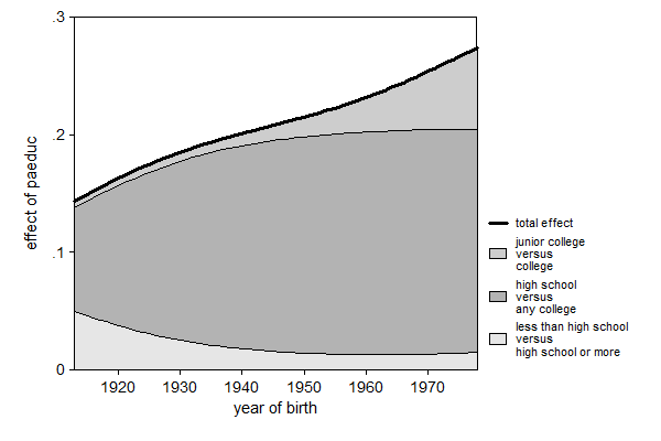
So in the oldest cohort a year increase in father's education was associated with about 0.15 years increase in the child's education. In the youngest cohort that effect almost doubled to about 0.27 years. The composition also changed quite a bit: Initially the transition whether or not to finish high school contributed a fair amount, but this has decreased. This decline has been more than compensated by the contribution of the transition whether or not to go to college, and for the most recent cohorts the choice between junior college and college has become a considerable contributor to the total effect of father's education.
The contributions of the transitions consist of two parts: a weight and an effect. This can also be visualized with seqlogitdecomp.
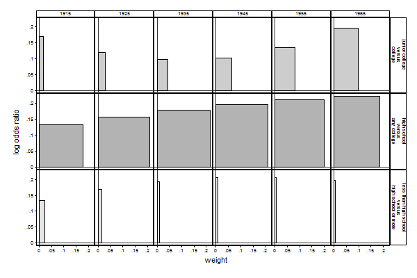
Graph 1b (Compare with Graph 2b). seqlogitdecomp, overat(coh -3.5, coh -2.5, coh -1.5, /// > coh -0.5, coh 0.5, coh 1.5) /// > at(south 0 paeduc 12 res16 3 sibs 1) /// > yline(0) xline(0) /// > subtitle("1915" "1925" "1935" "1945" "1955" "1965") /// > eqlabel(`""less than high school" "versus" "high school or more""' /// > `""high school" "versus" "any college""' /// > `""junior college" "versus" "college""' )
At:
variable | value -------------+--------- south | 0 paeduc | 12 res16 | 3 sibs | 1
Over:
variable | col 1 col 2 col 3 col 4 col 5 col 6 -------------+------------------------------------------------------ coh | -3.5 -2.5 -1.5 -.5 .5 1.5
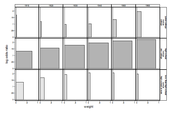
So, we can see that the decline in the contribution of the first transition is mainly due to the decline of the weight assigned to that transition, while the increasing contribution of the second and third transition is due to both an increase in the effect and an increase in the weight. This can be inspected in even more detail by using the table option in seqlogitdecomp:
Table 1a (Compare with Table 1b)Table 1b (Compare with Table 1a and Table 2). // decomposition for cohort born in 1965 . seqlogitdecomp paeduc, at(coh 1.5 south 0 paeduc 12 res16 3 sibs 1) table
At:
variable | value -------------+--------- coh | 1.5 south | 0 paeduc | 12 res16 | 3 sibs | 1
Decomposition:
| _1_2_3v0 | _2_3v1 | _3v2 | b se | b se | b se -------------+------------------+------------------+------------------ trans | | | paeduc | .197 .0242 | .221 .0146 | .197 .0251 -------------+------------------+------------------+------------------ weight | | | weight | .0654 .0123 | .862 .0144 | .196 .0162 at risk | 1 . | .987 .00255 | .542 .0197 variance | .0132 .00248 | .248 .00196 | .18 .0134 gain | 4.94 .0757 | 3.53 .051 | 2 . -------------+------------------+------------------+------------------ pr(pass) | | | pr | .987 .00255 | .549 .0199 | .764 .0255 -------------+------------------+------------------+------------------ tot | | | paeduc | .242 .25 | |
. // decomposition for cohort born in 1915 . seqlogitdecomp paeduc, at(coh -3.5 south 0 paeduc 12 res16 3 sibs 1) table
At:
variable | value -------------+--------- coh | -3.5 south | 0 paeduc | 12 res16 | 3 sibs | 1
Decomposition:
| _1_2_3v0 | _2_3v1 | _3v2 | b se | b se | b se -------------+------------------+------------------+------------------ trans | | | paeduc | .133 .0382 | .132 .0417 | .17 .0928 -------------+------------------+------------------+------------------ weight | | | weight | .344 .0815 | .741 .0564 | .0333 .013 at risk | 1 . | .909 .0236 | .274 .0346 variance | .0825 .0193 | .211 .0148 | .0606 .0223 gain | 4.17 .145 | 3.87 .0514 | 2 . -------------+------------------+------------------+------------------ pr(pass) | | | pr | .909 .0236 | .302 .0373 | .935 .0257 -------------+------------------+------------------+------------------ tot | | | paeduc | .149 .551 | |
If we look at the decomposition of the effect of father's education for the cohort born in 1915, we can see that the total effect is 0.149 years of education for every year increase in father's education, which is a weighted sum of the effects on each transition: 0.344×0.133 + 0.741×0.132 +0 .0333×0.17 = 0.149. The weight is in turn the product of its three components. Consider the first transition: 1×0.825×4.17 = 0.344. We can also see where these components come from: Everybody is by definition at risk for the first transition, so the proportion at risk is 1. The variance is 0.909×(1-0.909)=.083. Someone who passes the first transition can expect a 1-0.302 = 0.698 chance of attaining just high school, a 0.302×(1-0.935)=0.0196 chance of attaining junior college and a 0.302×0.935=0.282 chance of attaining college. So the gain of passing, that is, the expected level of education of those that pass minus the expected education of those that fail, is: 0.698×12 + 0.0196×14 + 0.282×16 - 9 = 4.17.
If we compare the cohort born in 1915 with the cohort born in 1965 we can see that the reason for the declining weight of the first transition is due to the fact that attaining a high school degree has become virtually universal for this group (male, white, not living in the south, a father with a high school degree, growing up in the suburbs with one sibling). This means that the variance has gone down from .0825 in 1915 to .0132 in 1965.
When it is not possible to assign values to each outcome
This decomposition of the effect on the final outcome into a weighted sum of effects on each transition worked because we had a scale on which to measure the final outcome: I assigned values, (pseudo-)years of education, to each level of education. The reason for that is that the effect on the final outcome is the slope of the curve of the expected outcome against the explanatory variable. If we cannot assign meaningful values to each outcome category, we cannot compute the expected value of the final outcome, and thus also not the effect on it.
However, there are many situations where one can meaningfully estimate a seqential logit but not assign meaningful values to all the outcomes. For example, consider the process of participating in a survey. First transition: whether or not a potential respondent was successfully contacted. Second transition: given that contact was made, whether or not a potential respondent chose to participate. In this case there are three outcomes: no contact, contact but not participate, contact and participate. In this case there is no equivalent of (pseudo-)years of education that can be used to assign meaningful values to each of these outcomes.
It is still possible to use this decomposition if there is one outcome of particular interest. In the survey participation example one can expect that this would be the "contact and participate" outcome. In that case we can assign the value 0 to both "no contact" and "contact but not participate" and the value 1 to "contact and participate" through the levels() option of seqlogit. That way the expected value of our outcome is the probability of being contacted and participating3.
We can use this trick to continue the example above by saying that we particularly care about whether or not someone gets a college degree. In that case we change the levels() from levels(0=9, 1=12, 2=14, 3=16) to levels(0=0, 1=0, 2=0, 3=1). The direct output of seqlogit will remain exactly the same, this change will only influence predict, any command that internally uses predict like margins, and seqlogitdecomp.
Graph 2a (Compare with Graph 1a). qui seqlogit degree south i.res16 c.sibs##c.sibs /// > c.coh##c.coh if black == 0 , or /// > tree(0 : 1 2 3 , 1 : 2 3 , 2 : 3 ) /// > ofinterest(paeduc) /// > over(c.coh##c.coh) /// > levels(0=0, 1=0, 2=0, 3=1)
. . seqlogitdecomp, area at(south 0 paeduc 12 res16 3 sibs 1) /// > xlab(-3 "1920" -2 "1930" -1 "1940" 0 "1950" 1 "1960" 2 "1970") /// > xtitle("year of birth") /// > eqlabel(`""less than high school" "versus" "high school or more""' /// > `""high school" "versus" "any college""' /// > `""junior college" "versus" "college""' )
At:
variable | value -------------+--------- south | 0 paeduc | 12 res16 | 3 sibs | 1
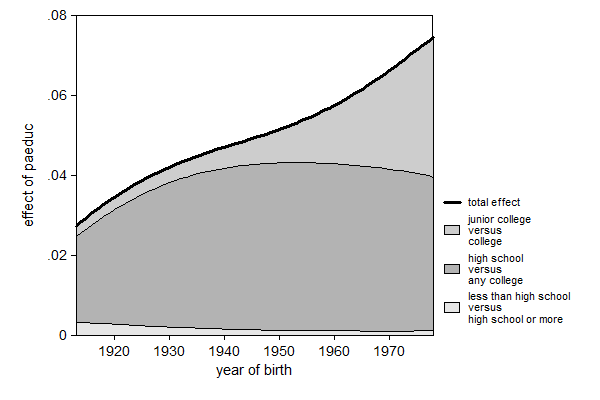
We can see in the graph above that a year change in father's education is associated with about a 3 percentage point4 increase in probability of attaining college for the cohort born in 1915 and about a 7 percentage point increase for the cohort born in 1975. Also notice that the transition whether or not someone finishes high school contributes less now that we only care about college graduation instead of years of education.
Given that the log odds ratios remain unchanged when the values assigned to each outcome change, the only way the effects can change is when the weights change. Comparing Graph 2b with Graph 1b shows that this is indeed the case.
Graph 2b (Compare with Graph 1b and Graph 3). seqlogitdecomp, overat(coh -3.5, coh -2.5, coh -1.5, /// > coh -0.5, coh 0.5, coh 1.5) /// > at(south 0 paeduc 12 res16 3 sibs 1) /// > yline(0) xline(0) /// > subtitle("1915" "1925" "1935" "1945" "1955" "1965") /// > eqlabel(`""less than high school" "versus" "high school or more""' /// > `""high school" "versus" "any college""' /// > `""junior college" "versus" "college""' )
At:
variable | value -------------+--------- south | 0 paeduc | 12 res16 | 3 sibs | 1
Over:
variable | col 1 col 2 col 3 col 4 col 5 col 6 -------------+------------------------------------------------------ coh | -3.5 -2.5 -1.5 -.5 .5 1.5
If we look at the detailed composition for the cohort born in 1915 using table option in seqlogitdecomp We can see that the only thing that changed is the gain component in the weight. Whether or not you finish high school is more important when one considers years of education instead of college completion because with years of education one assigns positive values to those with high school and junior college (compared with those with less than high school), while college completion deliberately ignores those gains.
Table 2 (Compare with Table 1b and Table 3). // decomposition for cohort born in 1915 . seqlogitdecomp paeduc, at(coh -3.5 south 0 paeduc 12 res16 3 sibs 1) table
At:
variable | value -------------+--------- coh | -3.5 south | 0 paeduc | 12 res16 | 3 sibs | 1
Decomposition:
| _1_2_3v0 | _2_3v1 | _3v2 | b se | b se | b se -------------+------------------+------------------+------------------ trans | | | paeduc | .133 .0382 | .132 .0417 | .17 .0928 -------------+------------------+------------------+------------------ weight | | | weight | .0233 .0062 | .179 .0143 | .0166 .00648 at risk | 1 . | .909 .0236 | .274 .0346 variance | .0825 .0193 | .211 .0148 | .0606 .0223 gain | .282 .0357 | .935 .0257 | 1 . -------------+------------------+------------------+------------------ pr(pass) | | | pr | .909 .0236 | .302 .0373 | .935 .0257 -------------+------------------+------------------+------------------ tot | | | paeduc | .0296 .018 | |
Using marginal effects instead of log odds ratios
In the examples above the effect on passing each transition was represented in log odds ratios. The main advantage of that is that this measure is less sensitive to changes in the transition rates across cohorts, making these effects more comparable across cohorts. However some prefer effect sizes in terms of marginal effects. The effect of explanatory variables on the final outcome can also be decomposed into a weighted sum of marginal effects on the probabilities of passing the different transitions. The reason is that the marginal effect on passing transition k is variancek (i.e. Prk[1-Prk]) times βk, so equation (2) can be rewritten as equation (3).
∂E(outcome)/∂x = ∑ ( at riskk × variancek × gaink ) βk (3)
= ∑ ( at riskk × gaink ) variancek × βk
=∑ ( at riskk × gaink ) marginal effectk
This has been implemented with the marg option for seqlogitdecom5. Continuing our example:
Graph 3 (Compare with Graph 2b). seqlogitdecomp, overat(coh -3.5, coh -2.5, coh -1.5, /// > coh -0.5, coh 0.5, coh 1.5) /// > marg /// > at(south 0 paeduc 12 res16 3 sibs 1) /// > yline(0) xline(0) /// > subtitle("1915" "1925" "1935" "1945" "1955" "1965") /// > eqlabel(`""less than high school" "versus" "high school or more""' /// > `""high school" "versus" "any college""' /// > `""junior college" "versus" "college""' )
At:
variable | value -------------+--------- south | 0 paeduc | 12 res16 | 3 sibs | 1
Over:
variable | col 1 col 2 col 3 col 4 col 5 col 6 -------------+------------------------------------------------------ coh | -3.5 -2.5 -1.5 -.5 .5 1.5
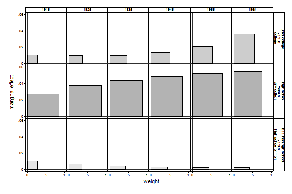
. // decomposition for cohort born in 1915 . seqlogitdecomp paeduc, at(coh -3.5 south 0 paeduc 12 res16 3 sibs 1) marg tab > le
At:
variable | value -------------+--------- coh | -3.5 south | 0 paeduc | 12 res16 | 3 sibs | 1
Decomposition:
| _1_2_3v0 | _2_3v1 | _3v2 | b se | b se | b se -------------+------------------+------------------+------------------ trans | | | paeduc | .011 .00261 | .0278 .00942 | .0103 .00562 -------------+------------------+------------------+------------------ weight | | | weight | .282 .0357 | .85 .0321 | .274 .0346 at risk | 1 . | .909 .0236 | .274 .0346 gain | .282 .0357 | .935 .0257 | 1 . -------------+------------------+------------------+------------------ pr(pass) | | | pr | .909 .0236 | .302 .0373 | .935 .0257 -------------+------------------+------------------+------------------ tot | | | paeduc | .0296 .018 | |
1 Or firms, countries, buffalo, or whatever your unit of analysis may be. [back]
2 See: Chapter 6, pages 109-112 of my dissertation. A more detailed step by step derivation is given in the appendix to that chapter. [back]
3 Remember that the expected value is just the average. If we have a set of observations that can only take the values 0 or 1, than the sum of these observations equals the number of 1s. When we divide the sum of these observations by the total number of observations we get the mean, which in this case is also the proportion of 1s. [back]
4 Notice the distinction between percentage change and percentage point change. A 10% increase when one starts with 10% is 11%, but a 10 percentage point increase when one starts with 10% is 20%. [back]
5 It is not possible to use the marg option together with the area option, like in graphs 1a and 2a, because these graphs show the total contribution of each transition, and these don't change, as is shown in equation (3). [back]