hangroot: module creating a hanging rootogram or suspended rootogram comparing an empirical distribution to a theoretical distribution
Author: Maarten L. Buis
hangroot creates a hanging rootogram or a suspended rootogram (Tukey 1973, 1977, Wainer 1974). The hanging rootogram compares a theoretical distribution with an empirical one, by "hanging" the histogram from the theoretical distribution, instead of "standing" the histogram on the x-axis. This way deviations are shown as deviations from a horizontal line (y=0) instead of deviations from a curve (the density curve). This makes it easier to spot patterns in the deviations. Also the y-axis is scaled as the square root of the frequency instead of the frequency to show deviations in the tails more clearly.
The suspended rootogram "suspends" the theoretical distribution from x-axis, basically flipping the hanging rootogram upside down. Moreover, it shows the residuals of the empirical distribution from the theoretical distribution rather than the entire histogram bars, which were shown in the hanging rootogram. The logic behind showing only the residuals is that they contain the key information telling us how well the theoretical distribution fits the empirical distribution, while the logic behind flipping the curve is that this way positive residuals means too many observation and negative residuals too few.
The user chooses the theoretical distribution with which (s)he wants to compare with the distribution of the variable, the parameter(s) of that distribution can also be fixed by the user or are/is chosen by hangroot to best fit the empirical distribution. hangroot allows one to compare the empirical distribution of a variable with one of the following theoretical distributions:
- normal / Gaussian (the default)
- lognormal
- logistic
- Weibull
- Chi square
- gamma
- Gumbel
- inverse gamma
- Wald / inverse Gaussian
- beta
- Pareto
- Fisk / log-logistic
- Dagum
- Singh-Maddala
- Generalized Beta II
- generalized extreme value
- exponential
- Laplace
- uniform
- geometric
- Poisson
Apart from comparing the distribution of a variable with one of the univariate distributions mentioned above it can also be used to compare the distribution of a variable with the marginal distribution implied by a regression model with covariates. In that case, the model assumes a distribution, but one or more parameters, typically the mean, can differ from observation to observation depending on the values of the covariates. The implied marginal distribution is a mixture distribution such that each observation has its own parameters.
This package can be installed by typing in Stata: ssc install hangroot
Supporting materials
- summary on ssc.
- helpfile
- Presentation held at the 2011 Nordic and Baltic Stata Users' meeting
- Initial announcement of hangroot on statalist, and announcements of the first, second, third, and fourth update of hangroot on statalist
References
John W. Tukey, 1972, Some Graphic and Semigraphic Displays. in: T.A. Bancroft and S.A. Brown, eds., Statistical Papers in Honor of George W. Snedecor. Ames, Iowa: The Iowa State University Press, pp 293-316. link
John W. Tukey, 1977, Exploratory Data Analysis, Addison-Wesley.
Howard Wainer, 1974, The Suspended Rootogram and Other Visual Displays: An Empirical Validation. The American Statistician, 28(4): 143-145.
Examples
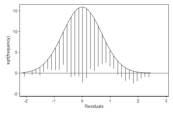
The hangroot package can be used to check distributional assumptions underlying a model. In the example below, the residual clearly deviates from the normal distribution as it is bi-modal.
. sysuse nlsw88, clear (NLSW, 1988 extract)
. gen ln_w = ln(wage)
. reg ln_w grade age ttl_exp tenure
Source | SS df MS Number of obs = 2229 -------------+------------------------------ F( 4, 2224) = 214.79 Model | 203.980816 4 50.9952039 Prob > F = 0.0000 Residual | 528.026987 2224 .237422206 R-squared = 0.2787 -------------+------------------------------ Adj R-squared = 0.2774 Total | 732.007802 2228 .328549283 Root MSE = .48726
------------------------------------------------------------------------------ ln_w | Coef. Std. Err. t P>|t| [95% Conf. Interval] -------------+---------------------------------------------------------------- grade | .0798009 .0041795 19.09 0.000 .0716048 .087997 age | -.009702 .0034036 -2.85 0.004 -.0163765 -.0030274 ttl_exp | .0312377 .0027926 11.19 0.000 .0257613 .0367141 tenure | .0121393 .0022939 5.29 0.000 .0076408 .0166378 _cons | .7426107 .1447075 5.13 0.000 .4588348 1.026387 ------------------------------------------------------------------------------
. predict resid, resid (17 missing values generated)
. hangroot resid (bin=33, start=-2.1347053, width=.13879342)
.
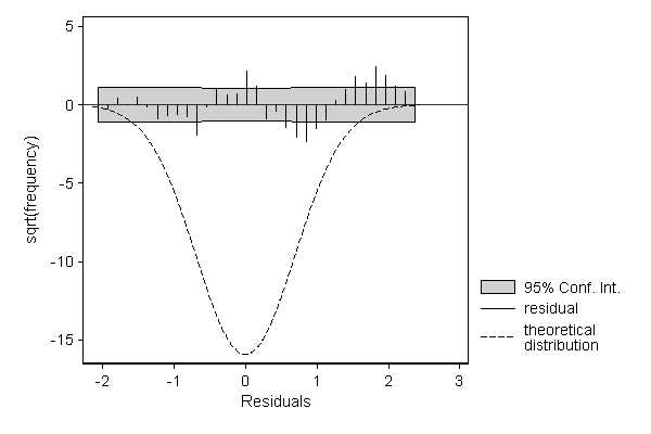
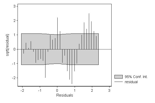
The deviations from the normal distribution are more clearly visible when displaying a suspended rootogram. Optionally, we can focuss entirely on these residuals by suppressing the display of the theoretical distribution.
. hangroot resid, susp theoropt(lpattern(-)) ci (bin=33, start=-2.1347053, width=.13879342)
. hangroot resid, susp notheor ci (bin=33, start=-2.1347053, width=.13879342)
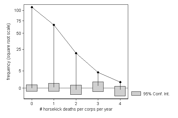
Sometimes the distribution of a variable has a direct substantive interpretation, as in the example from Bortkiewicz, L. (1898): Das Gesetz der kleinen Zahlen. Teubner, Leipzig. The point is to check whether death due to being kicked by a horse in different Prussian cavalry units occur randomly or whether some units are more skilled at avoiding kicks than others. If this is a random process, we would expect the number of deaths per unit to follow a Poisson distribution, which seems to be the case (as one would expect in a textbook example...).
This example also illustrates how regular graph options like ylab() and ytitle() can be used to improve the look of the graph.
. use http://fmwww.bc.edu/repec/bocode/c/cavalry.dta, clear (horsekick deaths in 14 Prussian cavalry units 1875-1894)
. hangroot deaths [fw=freq], /// > dist(poisson) ci /// > ylab(0 "0" /// > `=sqrt(5)' "5" /// > 5 "25" /// > `=sqrt(50)' "50" /// > `=sqrt(75)' "75" /// > 10 "100") /// > ytitle("frequency (square root scale)") (start=0, width=1)
.
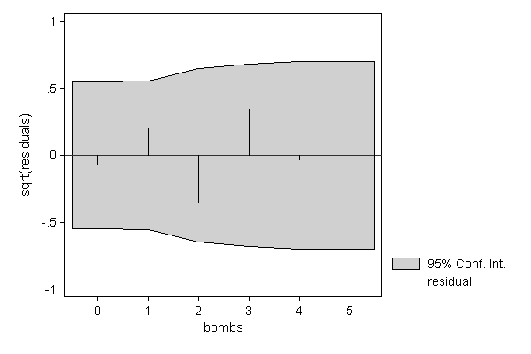
A similar example occurred in the Second World War when the British wanted to know whether flying bombs that where falling on London where aimed at specific sectors of the city or where falling randomly. An area of South London was divided into 576 squares of 1/4 square kilometer, and the number of bombs falling in each of them were counted. If the Germans could aim their bombs at specific areas within London we would expect the distribution to deviate from a Poisson distribution. The results appeared in R.D. Clarke (1946) "An application of the Poisson distribution" Journal of the Institute of Actuaries, 72:481. As can be seen below, there is no real deviation from the Poisson distribution, meaning that the Germans where able to steer their bombs to south London, but weren't able to aim them more precisely than that.
. drop _all
. input bombs areas
bombs areas 1. 0 229 2. 1 221 3. 2 93 4. 3 35 5. 4 7 6. 5 1 7. end
. . hangroot bombs [fw=areas], dist(poisson) susp ci notheor xlab(0/5) (start=0, width=1)
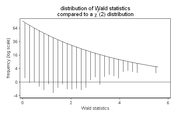
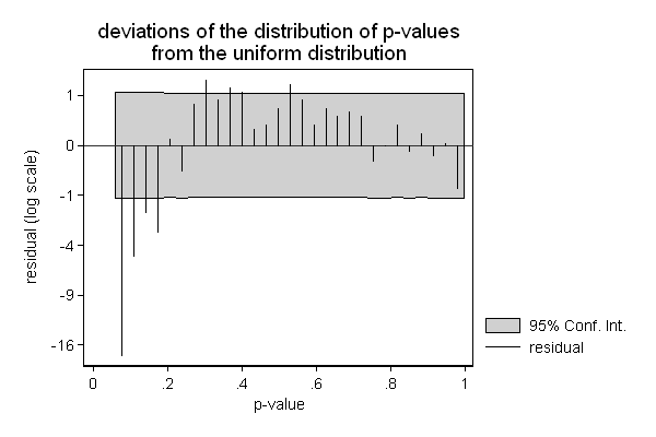
Another area where hangroot can be useful, is the presentation of the results of a simulation. In the example below, I am checking if the Wald test ( test in Stata) still performs well in a sample of only 25 observations. The background is that we know that this test may not perform well in small samples, and we wonder whether a sample size of 25 is too small.
In this case, we don't need to estimate the parameter of our theoretical distribution (the degrees of freedom): We know that the null hypothesis is true and that we are testing two constraints (the effect of x2 is 0 and the effect of x3 is 0), so the test-statistic should follow a chi square distribution with 2 degrees of freedom. So we use the par() option to fix the parameter of the theoretical distribution to 2. Similarly we know that the p-values should follow a uniform distribution ranging from 0 to 1.
The simulated sampling distribution does not seem to fit the theoretical sampling distribution well, so a sample size of 25 does appears to be too small for this test. (All is not lost, the Wald test seems to start to perform well with as few as 75 to 100 observations, while the likelihood ratio test ( lrtest in Stata) does appear to perform ok in samples as small as 25 observations.)
. program drop _all
. program define sim, rclass 1. drop _all 2. set obs 25 3. gen x1 = rnormal() 4. gen x2 = rnormal() 5. gen x3 = rnormal() 6. gen y = runiform() < invlogit(-2 + x1) 7. logit y x1 x2 x3 8. test x2=x3=0 9. return scalar p = r(p) 10. return scalar chi2 = r(chi2) 11. end
. . set seed 123456
. . // this will take a while. If you want some . // entertainment or an idea how far the . // simulation has progressed, remove the . // nodots option . simulate chi2 = r(chi2) p=r(p), reps(1000) nodots : sim
command: sim chi2: r(chi2) p: r(p)
. . hangroot chi2, dist(chi2) par(2) name(chi, replace) /// > title("distribution of Wald statistics" /// > "compared to a {&chi}{sup:2}(2) distribution" ) /// > xtitle(Wald statistics) /// > ytitle("frequency (log scale)") /// > ylab(-2 "-4" 0 "0" 2 "4" 4 "16" 6 "36" 8 "64") (bin=29, start=.00479837, width=.19250064)
. . hangroot p , dist(uniform) par(0 1) /// > susp notheor ci name(p, replace) /// > title("deviations of the distribution of p-values" /// > "from the uniform distribution") /// > xtitle("p-value") ytitle("residual (log scale)") /// > ylab(-4 "-16" -3 "-9" -2 "-4" -1 "-1" 0 "0" 1 "1" ) (bin=29, start=.06119692, width=.03228989)
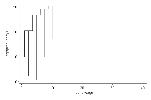
We can also use hangroot for comparing the distribution of variables across groups. In the example below the distribution of hourly wage is compared across people with and without a college degree. The wage distribution of people with a college degree plays the role of theoretical distribution and the wage distribution of people without a college degree "hangs" from it. As expected people with a college degree tend to earn more than people without a college degree.
. sysuse nlsw88, clear (NLSW, 1988 extract)
. hangroot wage, dist(theoretical collgrad) bin(15) (bin=15, start=1.0049518, width=2.6494425)
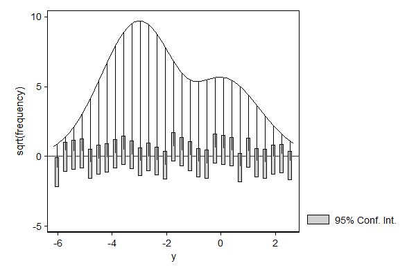
hangroot can also to compare the distribution of a variable against the marginal distribution implied by a regression model with covariates. If we add covariates to a model than we alow the parameters, typically the mean, to differ from observation to observation depending on these covariates. This means that the distribution of the dependent variable implied by the model is a mixture model of N distributions, such that each component distribution has the parameters of one of the observations in the data.
In this example there is only one binary variable, so the marginal distribution implied by our regression model collapses to a mixture of two components: one with a mean of -3 which applies to 3/4 of the observations and one with a mean of 0 which applies to 1/4 of the observations.
. set seed 1234
. drop _all
. set obs 1000 obs was 0, now 1000
. gen byte x = _n <= 250
. gen y = -3 + 3*x + rnormal()
. reg y x
Source | SS df MS Number of obs = 1000 -------------+------------------------------ F( 1, 998) = 1833.18 Model | 1751.98425 1 1751.98425 Prob > F = 0.0000 Residual | 953.794108 998 .955705519 R-squared = 0.6475 -------------+------------------------------ Adj R-squared = 0.6471 Total | 2705.77836 999 2.70848685 Root MSE = .9776
------------------------------------------------------------------------------ y | Coef. Std. Err. t P>|t| [95% Conf. Interval] -------------+---------------------------------------------------------------- x | 3.056782 .071394 42.82 0.000 2.916682 3.196881 _cons | -2.999406 .035697 -84.02 0.000 -3.069456 -2.929356 ------------------------------------------------------------------------------
. hangroot, ci (bin=29, start=-6.1794977, width=.30656038)