margdistfit: Post-estimation command that compares the observed and theoretical marginal distributions.
Author: Maarten L. Buis
margdistfit is a post-estimation command for checking how well distributional assumptions of a parametric regression model fit to the data. It does so by comparing the marginal distribution implied by the regression model to the distribution of the dependent variable. This comparison is done through either a probability-probability plot, a quantile-quantile plot, a hanging rootogram, or a plot of the two cumulative density functions.
The key concept in this command is the marginal distribution. The idea behind a parametric regression model is that it assumes a distribution for the dependent variable, and this distribution can be described in terms of a small number of parameters: e.g. the mean and the standard deviation in case of the normal/Gaussian distribution. One or more of these distribution parameters, typically the mean, is allowed to differ from observation to observation depending on the values of the explanatory variables. So, the marginal distribution of the dependent variable implied by the model is a mixture distribution of N distributions, such that each component distribution gets the parameters of one of the observations in the data.
To give an indication of how much deviation from the theoretical distribution is still legitimate, the graph will also show the distribution of several (by default 20) simulated variables under the assumption that the regression model is true. By default, the simulations include both uncertainty due to uncertainty about the parameter estimates and uncertainty due to the fact that they are random draws from a distribution. This is achieved by creating the simulated variables in two steps: first the parameters are drawn from their sampling distribution, and than the simulated variable is drawn given those parameters.
margdenfit may be used after estimating a model with regress or betafit.
This package can be installed by typing in Stata: ssc install margdistfit
Supporting materials
- summary on ssc.
- helpfile
- Presentation held at the 2011 Nordic and Baltic Stata Users' meeting
- Presentation held at the 2012 German Stata User's meeting
Examples
Table of content
Linear regression
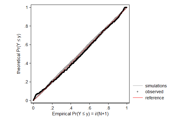
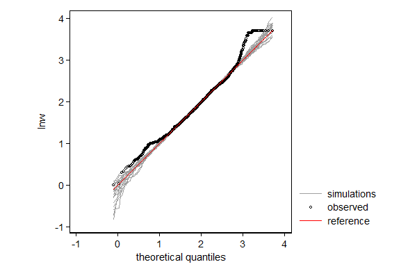
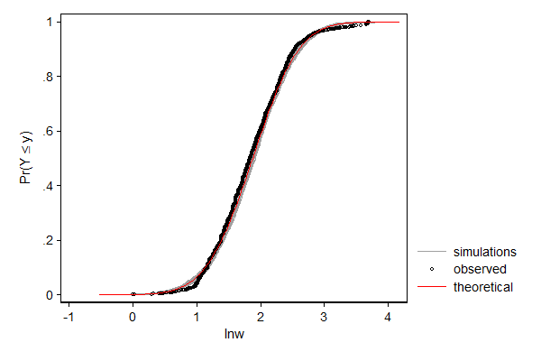
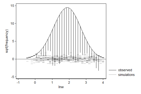
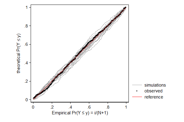
In the example below I model log hourly wage using linear regression. One can think of this as fitting a normal distribution to the data, but allow the mean to differ from observation to observation depending on the values of the explanatory variables. So the distribution of wage according to this model is a mixture distribution of N (in this case 2,229) normal distributions, such that each component distribution has a mean equal to the predicted log wage and a standard error equal to the root mean squared error/standard error of the estimate.
In case of linear regression the distributional assumption is not very important, but it can still be useful to spot patterns in the data that deviate from the model. In this case, the dependent variable does not match the theoretical distribution well in the right tail. One might investigate whether or not wage was top-coded, that is, whether all reported wages over a given cut-off value where assigned the cut-off value rather than the actual wage.
. sysuse nlsw88, clear (NLSW, 1988 extract)
. gen lnw = ln(wage)
. qui reg lnw i.race south grade c.ttl_exp##c.ttl_exp c.tenure##c.tenure
. . set seed 1234567
. margdistfit, pp refopts(lcolor(red))
. . set seed 1234567
. margdistfit, qq refopts(lcolor(red))
. . set seed 1234567
. margdistfit, cumul refopts(lcolor(red))
. . set seed 1234567
. margdistfit, hangroot(jitter(5)) (bin=34, start=-.52652043, width=.13520522)
.
beta regression
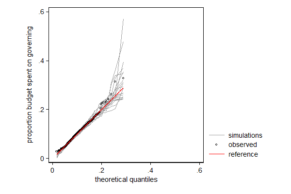
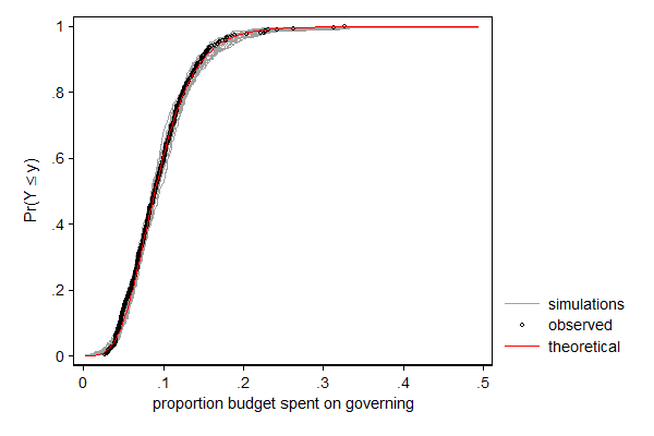
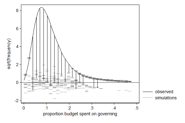
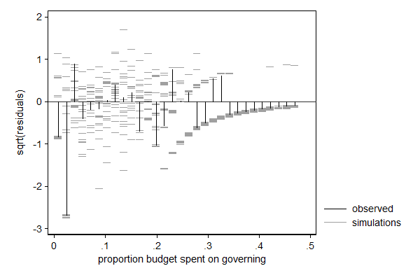
margdistfit can also be used after betafit, which fits a beta distribution. The beta distribution is a distribution for a bounded variable and is thus often used for modeling proportions. In the example below I model the proportions of its budget a city spends on its own organization with a beta distribution in which I let the mean and the scale parameter (mu and phi, respectively) depend on covariates. In this case it is the left tail that needs some attention: There are too few cases with very low proportions. Substantively that makes sense: there is a minimum larger than 0 under which that proportion in practice cannot go. For most application I would not consider this deviation too big of a problem, but if I would want to use this model to make statements on cities with very low proportions (presumably efficient cities) I would be a bit careful.
. use http://fmwww.bc.edu/repec/bocode/c/citybudget.dta, clear (Spending on different categories by Dutch cities in 2005)
. qui betafit governing , mu( minorityleft noleft popdens houseval) /// > phi(minorityleft noleft popdens houseval)
. set seed 1234567
. margdistfit, pp refopts(lcolor(red))
. . set seed 1234567
. margdistfit, qq refopts(lcolor(red))
. . set seed 1234567
. margdistfit, cumul refopts(lcolor(red))
. . set seed 1234567
. margdistfit, hangroot(jitter(5) start(1e-6) bin(30)) (bin=30, start=1.000e-06, width=.01591239)
. . set seed 1234567
. margdistfit, hangroot(susp notheor jitter(2) start(1e-6) bin(30)) (bin=30, start=1.000e-06, width=.01591239)
Count models
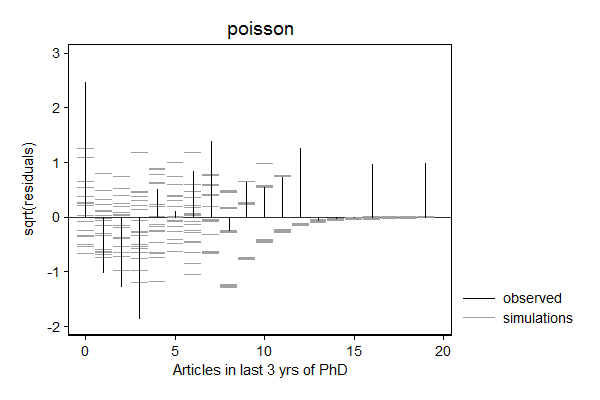
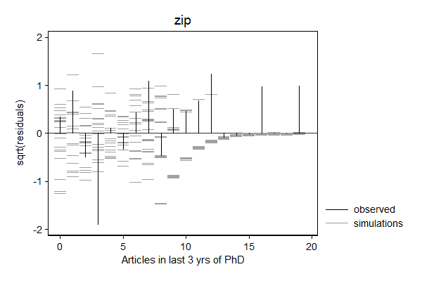
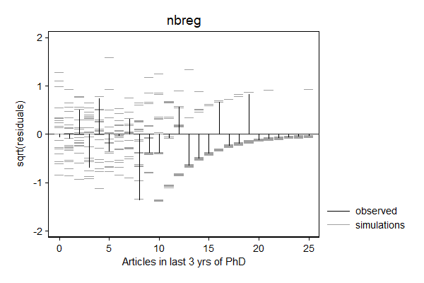
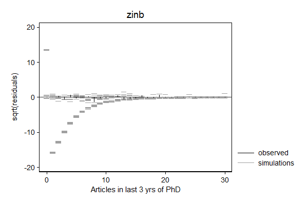
margdistfit can also help to choose between various count models, in particular poisson, zip, nbreg, and zinb. In the example below, the Poisson models does not do a good job predicting zeros and the tail, the Zero-inflated Poison does well with the zeros, but still struggles with the threes and the tail, the negative binomial seems to do a good job, while simulated values from the zero inflated negative binomial look "weird".
Looking back at the parameter estimates these weird simulations can be explained by the fact that the inflate probability is extremely imprecisely estimated. The simulations are performed by first drawing a new set of "parameters" from the sampling distribution of the parameters, and than sampling from that new distribution. The extreme imprecision of the inflate probability means that half the samples will be from a distribution with only a spike at 0 while the other half will be from a negative binomial distribution without any inflation at 0. The weird pattern in the simulations are in this case a sign that the zero inflated negative binomial distribution is not a good model for this data.
So in this case, the negative binomial seems to fit best.
. use http://www.stata-press.com/data/lf2/couart2,clear (Academic Biochemists / S Long)
. mkspline ment1 20 ment2 = ment
. . poisson art fem mar kid5 phd ment1 ment2, nolog
Poisson regression Number of obs = 915 LR chi2(6) = 214.34 Prob > chi2 = 0.0000 Log likelihood = -1635.404 Pseudo R2 = 0.0615
------------------------------------------------------------------------------ art | Coef. Std. Err. z P>|z| [95% Conf. Interval] -------------+---------------------------------------------------------------- fem | -.2256257 .0546189 -4.13 0.000 -.3326767 -.1185747 mar | .155161 .0612854 2.53 0.011 .0350438 .2752781 kid5 | -.1691524 .0400504 -4.22 0.000 -.2476498 -.090655 phd | -.0219537 .0273412 -0.80 0.422 -.0755414 .031634 ment1 | .047602 .0044176 10.78 0.000 .0389436 .0562603 ment2 | .0072431 .0041885 1.73 0.084 -.0009661 .0154524 _cons | .2410454 .1040761 2.32 0.021 .03706 .4450309 ------------------------------------------------------------------------------
. margdistfit, hangroot(susp notheor jitter(2)) title(poisson) (start=0, width=1)
. . zip art fem mar kid5 phd ment1 ment2, inflate(_cons) nolog
Zero-inflated Poisson regression Number of obs = 915 Nonzero obs = 640 Zero obs = 275
Inflation model = logit LR chi2(6) = 145.07 Log likelihood = -1606.858 Prob > chi2 = 0.0000
------------------------------------------------------------------------------ art | Coef. Std. Err. z P>|z| [95% Conf. Interval] -------------+---------------------------------------------------------------- art | fem | -.2366895 .0580148 -4.08 0.000 -.3503965 -.1229826 mar | .1395344 .0653419 2.14 0.033 .0114666 .2676021 kid5 | -.1566819 .0428666 -3.66 0.000 -.2406989 -.0726648 phd | -.0378266 .0296474 -1.28 0.202 -.0959344 .0202812 ment1 | .0449336 .0048883 9.19 0.000 .0353526 .0545146 ment2 | .0042559 .0042506 1.00 0.317 -.0040752 .0125869 _cons | .4756723 .1144958 4.15 0.000 .2512646 .70008 -------------+---------------------------------------------------------------- inflate | _cons | -1.803867 .1692401 -10.66 0.000 -2.135572 -1.472163 ------------------------------------------------------------------------------
. margdistfit, hangroot(susp notheor jitter(2)) title(zip) (start=0, width=1)
. . nbreg art fem mar kid5 phd ment1 ment2 , nolog
Negative binomial regression Number of obs = 915 LR chi2(6) = 111.15 Dispersion = mean Prob > chi2 = 0.0000 Log likelihood = -1554.3612 Pseudo R2 = 0.0345
------------------------------------------------------------------------------ art | Coef. Std. Err. z P>|z| [95% Conf. Interval] -------------+---------------------------------------------------------------- fem | -.2122617 .0720599 -2.95 0.003 -.3534965 -.071027 mar | .1584807 .0814731 1.95 0.052 -.0012037 .3181651 kid5 | -.1668426 .0526027 -3.17 0.002 -.269942 -.0637432 phd | -.0105595 .0363468 -0.29 0.771 -.0817978 .0606789 ment1 | .0475126 .0061049 7.78 0.000 .0355472 .059478 ment2 | .0070301 .0067191 1.05 0.295 -.0061392 .0201993 _cons | .1974055 .1381738 1.43 0.153 -.0734102 .4682212 -------------+---------------------------------------------------------------- /lnalpha | -.8702071 .1242129 -1.11366 -.6267542 -------------+---------------------------------------------------------------- alpha | .4188648 .0520284 .328355 .5343233 ------------------------------------------------------------------------------ Likelihood-ratio test of alpha=0: chibar2(01) = 162.09 Prob>=chibar2 = 0.000
. margdistfit, hangroot(susp notheor jitter(2)) title(nbreg) (start=0, width=1)
. . zinb art fem mar kid5 phd ment1 ment2, inflate(_cons) nolog
Zero-inflated negative binomial regression Number of obs = 915 Nonzero obs = 640 Zero obs = 275
Inflation model = logit LR chi2(6) = 111.15 Log likelihood = -1554.361 Prob > chi2 = 0.0000
------------------------------------------------------------------------------ art | Coef. Std. Err. z P>|z| [95% Conf. Interval] -------------+---------------------------------------------------------------- art | fem | -.2122618 .0720599 -2.95 0.003 -.3534965 -.071027 mar | .1584807 .0814731 1.95 0.052 -.0012037 .3181651 kid5 | -.1668426 .0526027 -3.17 0.002 -.269942 -.0637432 phd | -.0105595 .0363468 -0.29 0.771 -.0817978 .0606789 ment1 | .0475126 .0061049 7.78 0.000 .0355472 .059478 ment2 | .0070301 .0067191 1.05 0.295 -.0061392 .0201993 _cons | .1974055 .1381738 1.43 0.153 -.0734102 .4682212 -------------+---------------------------------------------------------------- inflate | _cons | -24.95389 42277.72 -0.00 1.000 -82887.76 82837.85 -------------+---------------------------------------------------------------- /lnalpha | -.8702071 .1242129 -7.01 0.000 -1.11366 -.6267542 -------------+---------------------------------------------------------------- alpha | .4188648 .0520284 .328355 .5343233 ------------------------------------------------------------------------------
. margdistfit, hangroot(susp notheor jitter(2)) title(zinb) (start=0, width=1)